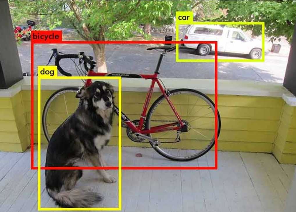
There are three main applications of AI. Images, data, and language. The image processing includes several tasks such as image classification, image dimension reduction, image generation, style transfer, object detection and segmentation. The object detection is a function that feeds image as input, and output several bounding boxes with its image class and confidence, which commonly used in monitoring.
The main stream object detection algorithms includes FasterRCNN, SSD and Yolo. In this article, you will learn the fundamental principle of Yolo version 3, its environment installation and the implementation.
Theory
network structure
Yolo which is an end-to-end neural network for the object detection which has the following structure.
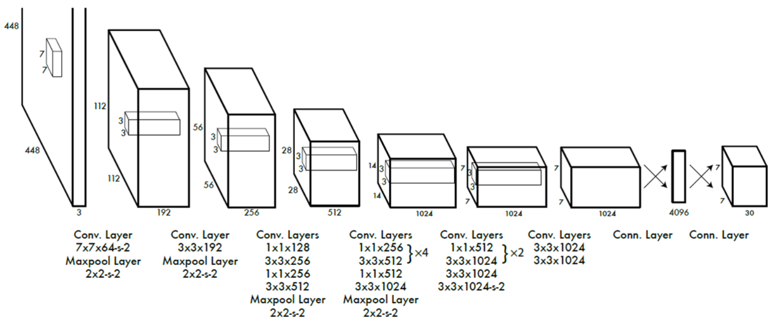
As if the CNN model, the input layer is an image with size 448×448×3 followed by several convolutional layers, max-pooling layers, and dense layers. These layers plays a role for feature extraction and classification. The main difference is the output layer which reshape the neuron back to 3 dimensions. Let’s discuss about the meaning of it.
A N×N images can be equally divided into S×S grids with N/S × N/S for each. Next, a hyperperameter B determines the number of bounding box centers for each grid. That is, we will see at most B bounding box center in each grid. The more B is, the higher accuracy will be obtained but performance decreased on the contrary. A bounding box holds 5 parameters, center coordinate (x,y), width w, height h, and the confidence c belongs to a class. Finally, the number of classes we want to detect is another hyperparameter C. The output class is one-hot-encoded, therefore, the output of entire neural network has the shape
1 | S×S×(B×5+C). |
The original example proposed by the author set N=448, S=7, B=5, C=20 and used VOC as dataset.
Confidence, IOU
Although it predict B bounding boxes in a grid, there are only a predicted probability P(object-in-grid) that describe the prob for an object existing in the grid. The confidence score regardless of image classification for each bounding box is c=P(object-in-grid)*IOU
, where IOU stands for intersection over union and represents the similatiry or overlapping between predicted bounding box and true bounding box. However, each bounding box also recognize a class, so the overall confidence score for a bounding box is
1 | c = P(class-i|object-in-grid)*P(object-in-grid)*IOU = P(class-i)*IOU. |
It is more intuitive and elegant as well as combine the classification trem P(class-i) and regression (location) term IOU. Furthermore, as soon as a predicted bounding box generated, we only need to calculate the IOU between itself and the true bounding box belongs to the grid. Hence, Yolo can solves the object detection efficiently.
Non-Maximum Suppression (NMS)
Moreover, NMS is an algorithm that filter the redundant bounding boxes which is indispensable in object detection algorithms.
- sort all the bounding boxes according to their confidence score and initialize an empty result list.
1
2
3
# example
candidates=[B1,B2,B3,B4,B5]
result=[] - Move
candidates[0]to Result.1
2candidates=[B2,B3,B4,B5]
result=[B1] - Calculate the IOU between
Result[-1]and each element in candidates.1
2
3candidates=[B2,B3,B4,B5]
result=[B1]
IOU=[0.3,0.7,0.4,0.1] - Remove all the bounding boxes that IOU>0.5 from candidates.
1
2candidates=[B2,B4,B5]
result=[B1] - Go back to step 2 until candidates is empty
Improved version
The improved version of Yolo have been proposed to fourth version so far. The improvment points includes
- Higher solution with 416×416×3 shape in input layer
- Anchor box convolution
- k-means for bounding boxes
- Residual net
Environment Setting
System requirements
- Anaconda
- Python=3.5
- Tensorflow=1.6 or Tensorflow-gpu=1.6
- Keras=2.1.5
- (optional) GPU environment
- Create an virtual environment for python=3.5 with name yolov3 for instance. Then install the above requirement.The labelImg is a free tool that help us to do the labeling for object detection conveniently. The labeling of a image in object detection problem includes several bounding box with its belongs class.
1
2
3
4conda create -n yolov3 python=3.5
conda activate yolov3
python -m pip install --upgrade pip
pip install labelImg pillow tensorflow==1.6 keras==2.1.5 matplotlib h5py - Create a directory and open CMD. Then, use git to clone the framework.
1
git clone https://github.com/OmniXRI/OpenVINO_RealSense_HarvestBot
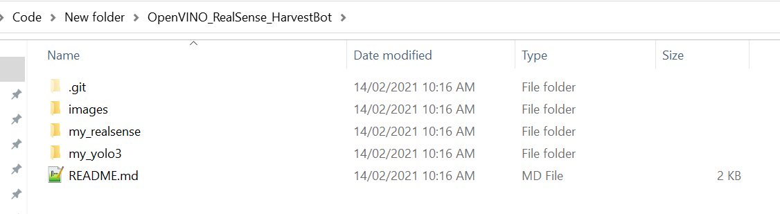
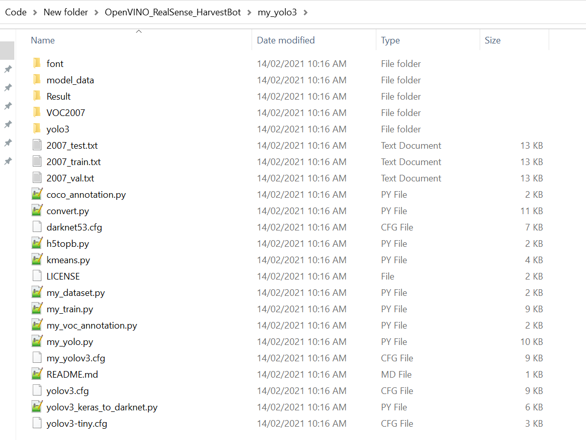
Not all the files cloned from github will be used. To make it simpler, move all the files in the foldermy_yolo3to the New folder and delete the others. - Download the weight to the folder. So all the files are same as the following.
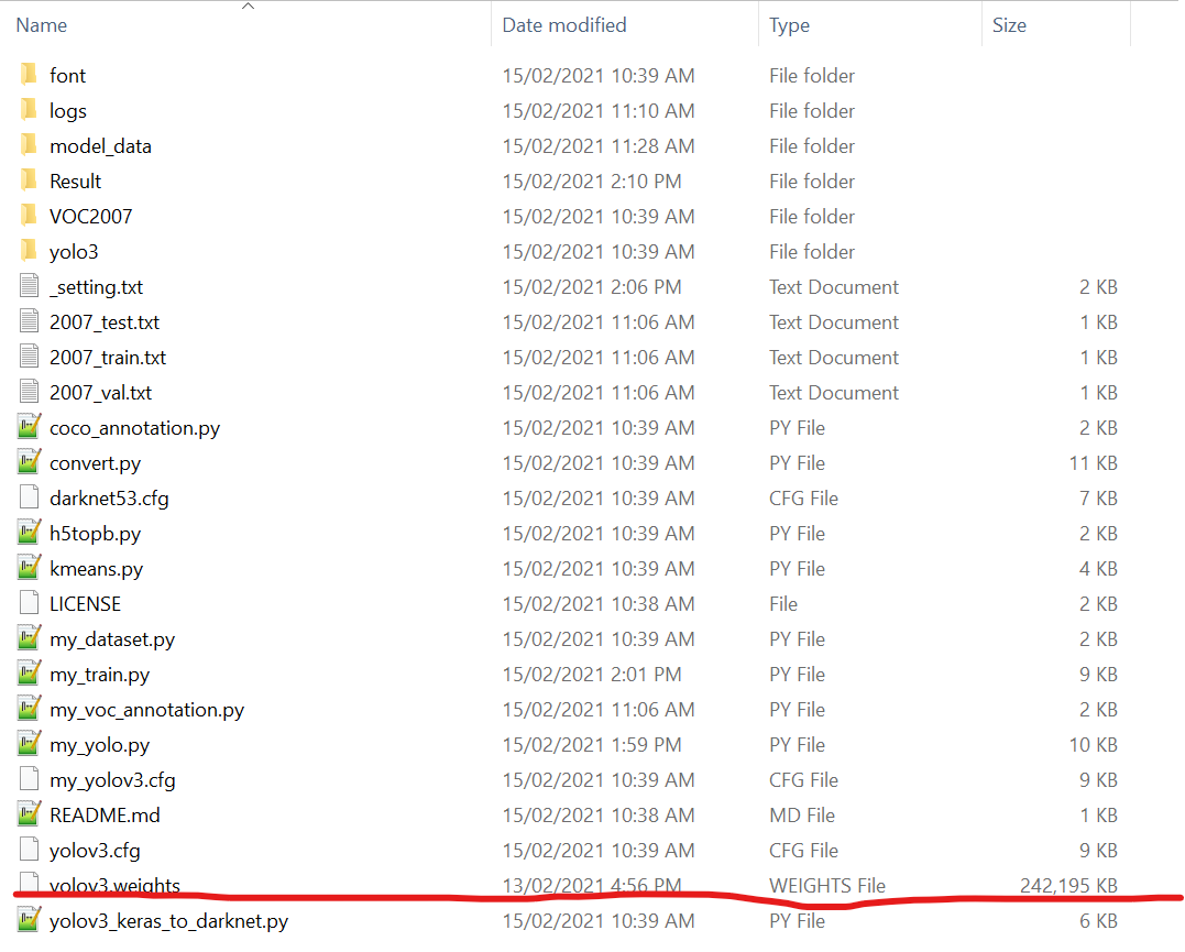
- Convert the weight to the format for Keras.
1
python convert.py -w yolov3.cfg yolov3.weights model_data/yolo_weights.h5
Implementation
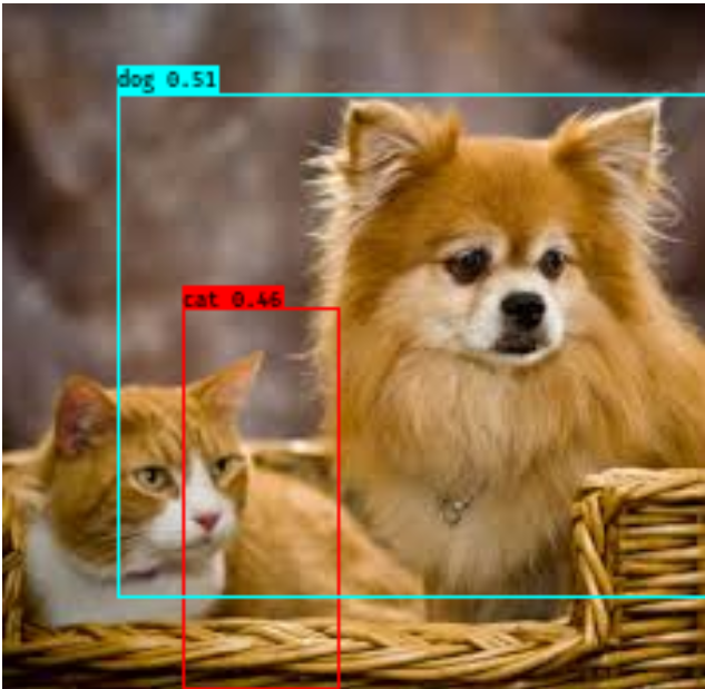
Here I download 20 pictures of cats and dogs. The goal is to do the two classes object detection for them.
Put the images into
VOC2007/JPEGImages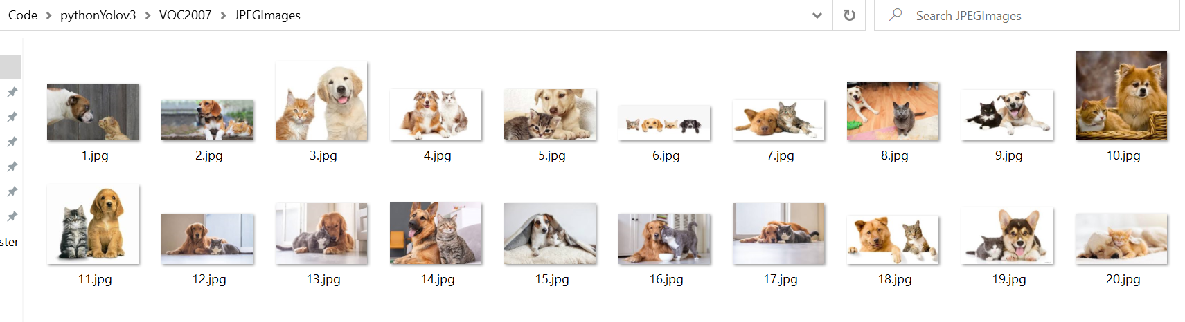
Launch the labeling tool in terminal.
1
labelImg
Click “change save directory” and specify the folder “VOC2007/JPEGImages”. Next, click “open directory” and specify the folder “VOC2007/Annotations”. Now, we can label all the images (press
wto start labeling), and you will see the output format.xmlin “VOC2007/Annotations”.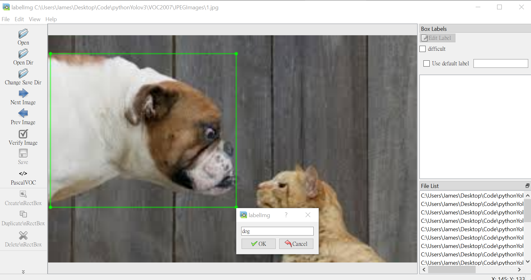
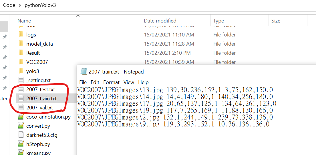
Execute
python my_dataset.py. It will load the annotations and random generate the train index, val index, test index in “VOC2007/ImageSets/Main”.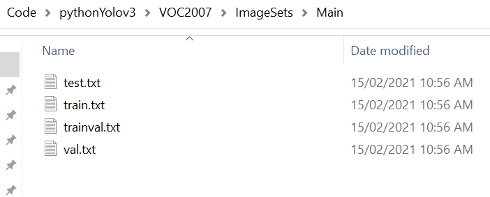
Modify
model_data/my_classes.txt. Change the classes to dog and cat.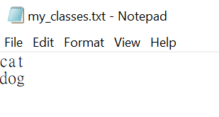
Modify same thing in line 6 of
my_voc_annotation.py. Then executepython my_voc_annotation.pyto generate the data with labels.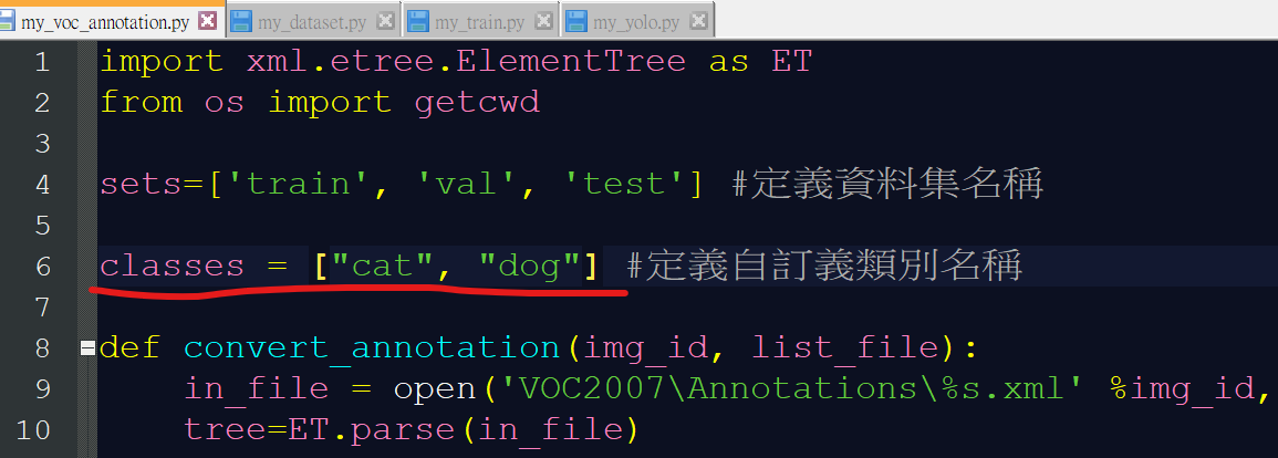
Open the
my_train.pyand setting some parameters before training.- modify the weights path to “model_data/trained_weights_stage_1.h5” in line 32 if you are doing transfer learning (skip this step first time).
- delete callback in line64
- change True to False in line69
- change epoch and learning rate if needed (you can set epoch=1 for first time)
We can start training now.1
python my_train.py
During the training, we can modify the predicting script
my_yolo.py. The only one thing need to change is the path in line 216.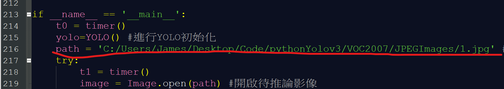
After the training finish, we can see the weightlogs/000/trained_weights_stage_1.h5. Bring the weight to the folder model_data.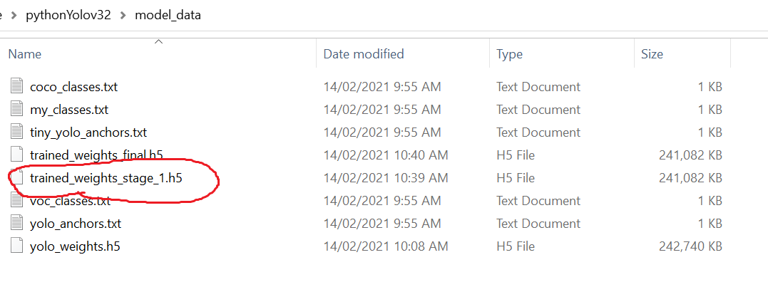
Finally execute the inference script to obtain the result.
1
python my_yolo.py
If the result is not well, go back to the step 7 and doing transfer learning.